
Hold the front page, Doug Keenan has a confession from the Met Office that “statistically significant temperature rise can’t be supported”.
In a long post, more concerned with the details of which minister would not answer which parliamentary question than the statistics, Keenan gloats over extracting from the Met Office the admission that an ARIMA(3,1,0) model explains global temperature change in the instrumental record better than a linear trend with autocorrelated (AR1) residuals, and hence he declares that the rise in temperatures is not significant.
Keenan assures the reader that “unfamiliarity with the model does not matter here”. I would demur, model choice on purely statistical criteria is a empty pursuit of meaningless models. If we do not understand what the models are doing, we cannot evaluate if the models are sensible.
The linear trend model fits a regression to the data, but rather than assuming that the residuals from this regression are independent, they are expected to be autocorrelated. That is neighbouring residuals are expected to be more similar than residuals selected at random.
Keenan would have us replace this model with ARIMA(3,1,0), an autoregressive integrated moving average model. The 3 designates the number of terms in an autoregressive model. This is not dissimilar to the first model that expected the residuals to be from a first order autoregressive model. More interesting is the second number, 1, which indicated the number of times that the data must be differenced (subtracting the temperature of the previous year from the temperature of the current year) to make the data stationary, ie trendless.
Yes, Keenan argues there is no trend in the data by using a method that removes trends from data. By demonstrating that a differencing is needed, Keenan demonstrates there is a trend in the data. Whether this trend is accounted for by a linear trend or a differencing operation is a choice. Neither carry much physical meaning.
So lets have a look at applying his ARIMA(3,1,0) model to the Met Office data. First we import and plot the data and the differenced data.
had<-read.table("http://www.metoffice.gov.uk/hadobs/hadcrut4/data/current/time_series/HadCRUT.4.2.0.0.annual_ns_avg.txt")[,1:2]
names(had)<-c("year", "temperature")

x11(6,4);par(mgp=c(1.5,.5,0), mar=c(3,3,1,1), mfrow=c(1,2))
plot(had, type="l")
plot(diff(had$temp), type="l")

Global temperatures (left) and differenced global temperatures (right)
The strong trend in the left-hand plot is obvious. The right-hand plot shows no trend — the differencing operation has removed it — and the data lack strong autocorrelation. An ACF plot of the differenced data confirms this, there is weak negative autocorrelation for two or three lags.
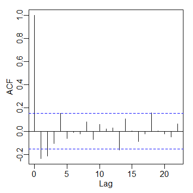
ACF of differenced global temperature data.
We can then fit the ARIMA(3,1,0) model to the raw data, or equivalently, an ARIMA(3,0,0) model to the differenced data.
acf(diff(had$temp))

mod1<-arima(had$temp,order=c(3,1,0))
mod2<-arima(diff(had$temp),order=c(3,0,0), include.mean=F)
The three AR coefficients are all small and negative (-0.38,-0.37, and -0.27), and their physical meaning is not obvious.
We can test if Keenan’s model is a plausible representation of climate by simulating a Holocene-length time series. The Holocene is known to have a rather stable climate, can this model simulate that?
sims<-replicate(5,{
  arima.sim(list(order=c(3,1,0), ar=coef(mod1)),10000, sd=sqrt(mod1$sigma2))
})
matplot(sims, xlab="year", ylab="temperature anomaly °C", type="l", col=1:5, lty=1)

Five Holocene-length realisations of an ARIMA(3,1,0) process
That I think is a NO! In these simulations, there are up to 15°C of global temperature change, rather larger than the actual ~1°C change in the Holocene. All the realisations have more temperature change than the glacial-interglacial temperature difference. But perhaps the climate is usually stationary, maybe from an ARIMA(3,0,0) process, and the non-stationarity that needs differencing only occurs during the last 150 years. What could possibly have caused this non-stationarity, this trend during the last 150 years? It couldn’t be greenhouse gases could it?
 @richardjtelford

Interesting analysis.
Are the Met Office statisticians not up to doing time series analysis – would you say?
I am sure the Met Office statisticians are doing an excellent job, but probably have limited patience with Keenan’s valiant attempts to prove that it is not warming.
An earlier post on Bishop Hill states that Keenan has had: “cordial e-mail discussions in the past. In particular, after my op-ed piece in WSJ appeared, on 12 August 2011, McNeall sent me an e-mail stating that the trending autoregressive model is “simply inadequate”. Indeed, that would be obvious to anyone who has studied statistical time series at the undergraduate level. Note that this implies that a statistician at the Met Office has stated that the Answer given to the original Parliamentary Question (HL3050) is unfounded.”
http://www.bishop-hill.net/blog/2013/4/9/questions-to-ministers.html
Perhaps you saw that?
Could I suggest that you post a summary of your analysis and a link to this blog at the current Bishop Hill blogpost, and see what response you get. It would be useful to get Keenan’s response, in particular.
A quick glance at the residuals from the linear trend is enough to know that there the residuals are non-stationary, and that AR1 is not sufficient. I don’t think this is at all surprising: climate forcing has not increased linearly, so it is not reasonable to expect temperature to have increased in a linear fashion.
The linear trend model can certainly be improved, but the conclusion that it is warmer now than a century ago is not in doubt.
Obviously temp has increased, but question is whether this is just natural variability or driven?
Also question as to why temp increase has stalled for the last 15 yrs despite large increases in CO2.
The linear trend analysis cannot demonstrate causality – it does not even try. Keenan’s analysis assumes that the data follow a random walk, which violates the laws of thermodynamics (Lucia). Greenhouse gas forcing is certainly large enough to account for a large fraction of the warming, solar activity a lesser fraction.
Since 1998 there has not been a large El Niño event. When the next large El Niño occurs, global temperatures will probably reach record values. And then the sceptics will reset their clocks and start again – no warming for one year, no warming for two years…
The natural-vs-driven question is essentially settled via roughly a dozen attribution studies over the past decade and more, not one of which has found natural variability adequate to explain the data.
Short-term apparent pauses, such as we now appear to be in the midst of, are an inevitable result in any time series dataset where the signal-to-noise ratio is low. See, e.g., Skeptical Science’s “escalator” graphic: http://www.skepticalscience.com/graphics.php?g=47
Pingback: Musings on Quantitative Palaeoecology
I’m curious about the trend component in the ARIMA(3,1,0) and in particular how it is reflected in the simulation you ran. How come the big dip from 3000 to 5000 when you have a trend in the order of +0.01 per year (as I presume you have)?
The simulation plots have been redrawn since you wrote this. If you ignore the rather small AR coefficients, the ARIMA model is a Gaussian random walk. It is the cumulative sum of random numbers from a Normal distribution. There is no underlying trend in the simulation, the expected change at each time-step is zero, and the direction of change is as likely to be positive as negative.
There is around a 1 in 60 chance that a purely random model (integers between -20 and 20 with an 11 year running average) will produce (with over 50% accuracy) the last 90 years of gistemp.
Therefore, during the last 11,000 years, it is almost certain that a period of warming and character like that of the 20th century (with warming up to 1940, then stasis until 1975, then a resumption of warming, etc..) occurs around “twice” (every 5340 years).
So the real question is whether global warming random? I have just demonstrated that fitting a random model that not only reproduces the magnitude of warming, but the character of temperature change during that period, is indeed possible (however unlikely).
What do you think the likely hood would be when simply matching a period whose magnitude is similar, and ignoring the character of the warming? Can the global warming people please stop pretending they can prove global warming is not random!
Sure, some rare sets of random numbers will by chance resemble an observed dataset, but if only 1 in 60 have a good match, it would suggest that the observed temperature record is unlikely under your null hypothesis. I would strongly argue that your null hypothesis is physically unreasonable.
Agree, but more like 1 in 10 for magnitude (being very generous, some rare sets of numbers really put recent warming to bed), remember the hockey is around 1000 years long and surprise surprise there is a warming uptick (right on average?). There are no physics in the example, it simply demonstrates that it is possibly random. Expert judgment on the likely hood of AGW is simply (like most of the peer reviewed literature on this issue) opinion, rather than empirical evidence. As long as it is open to interpretations of assumptions based on yet more assumptions, then there will be skeptics (and rightly so.)
For the record I believe there should be reductions because contrary to alarmists, reductions should be based on the fact that we don’t know what will happen. However, to be perfectly honest I only hold that position because I feel it will not last very long.
🙂
There has never been a statistical test in any subject where the result was so extreme that it could not possibly have been due to chance.
Concern about greenhouse gases is not predicated on the instrumental record, but on the radiative properties of the gases.
You know there is famous statement made by feymann to his students, regarding a random number plate in a car park (i.e whats the chance of that?) An incredibly –unlikely– “construct”.. When your busy “making stuff up”, everything can seem unlikely!
There is a reason why authority (the met office for a recent example) clings to “fundamental physics”. It’s because they have the best idea of the physics of today, which, in regards to climate change, is very likely to be wrong. Sometimes it’s OK to admit ignorance.
Imperfect knowledge does equate to complete ignorance. Waiting until knowledge is perfect and uncertainty zero (if these are even possible) means waiting until we are committed.
I find it somewhat confusing why anyone would think a linear trend is adequate to fit the decidedly non-linear pattern of change in the level of the global NH temperature data. You’d need a reasonably complex ARMA model to capture the deviations from linearity, when a relatively simple model that assumes the level of the series varies smoothly does the job just as well.
Yes, Keenan is attaching a strawman hypothesis.
I had seen your comments at Bishop Hill and Watts Up With That, and assumed you were trolling; so I did not respond. Seeing this post now, I will give a short reply.
The ARIMA model is specified to be driftless: this means that the drift (i.e. average of the first differences of the series) in the model is 0. Your claim that differencing the series removes a trend makes no sense: if there was a trend, the drift would obviously not be 0.
My post did not claim that the ARIMA model should be used for drawing statistical inferences about the temperature series–contrary to your representations. The result reported in the post is strictly negative: i.e. the claim that the increase in temperatures is significant is unfounded.
The linear trending model was not advocated by me; rather, it was adopted by the IPCC, and this is discussed (with linked references) in my post. The Met Office was following the IPCC.
For anyone interested in this topic, I recommend reading my original post at Bishop Hill, my op-ed piece in the Wall Street Journal, and the comments that I left in this post:
http://www.bishop-hill.net/blog/2013/5/27/met-insignificance.html
The mean of the differenced data is not zero. It is 0.005. There is a trend in the data, the differencing step removes it.
The mean of the differences is not going to be exactly zero, with a stochastic process. By your reasoning, if we flip a coin 100 times and it comes up heads 51 times, that proves that the coin is not a fair coin.
More generally, in statistics, inferences are not drawn directly from the data. Rather, a statistical model is fit to the data and then inferences are drawn from the model. The question is this: what model should be selected? The IPCC selected a particular model (a straight line with AR(1) residuals); the Met Office followed that. I showed that their selection is untenable. I did not, though, advocate selecting any particular model.
The standard reference for this area is Model Selection by Burnham & Anderson (2002). The book currently has about 20000 citations on Google Scholar:
http://scholar.google.co.uk/scholar?cites=7412663974370808272
–which seems to make it the most highly-cited statistical research work published during the past quarter century. The second author, David Anderson, is listed in the Acknowledgements section of my op-ed piece, as he confirmed my methods.
Your previous comment presented a simple test: “if there was a trend, the drift would obviously not be 0.” It was that to which I was responding. Obviously there is a trend in the data, it is warmer now than in the 1850s. Describing this trend is a useful way to summarise the data. Nobody is surprised that the increase in temperature does not follow a linear trend, because the climate forcing is not linear, so demonstrating that an arbitrary, unphysical model performs better than a linear trend is to savage a straw man.
It is trivially easy to demonstrate that your test is hopelessly sensitive to deviations from a linear trend. It is not fit for purpose.
Of course what any good experiment needs is replication and controls. If the temperature had gone up consistently in the replicate planets, then it would be easy to reject the null hypothesis. Unfortunately, we lack replicates (and controls which would be very useful as refuges): we need physically-realistic attribution studies based on our single replicate, not unphysical null model tests.
By differencing in your ARIMA fit you are affectively fitting an ARMA(3,0) in the first-differenced time series. By differencing the series you are then fitting a model for the “residuals” about this “differenced trend”. Hence in that sense your model is for the stochastic properties about the “trend”, not for the data series themselves. I.e. you a fitting a model to the right hand panel in Richard’s post above, not the data in the left-hand panel.
Your claim that as the ARIMA(3,1,0) fits the data a lot better than the linear regression with AR(1) errors it should be preferred over the latter is also odd; you’d at least have to show that it did give an adequate fit to the data too. I don’t know if that statement was made simple for purposes of brevity (God knows the rest of the post on Bishop-Hill was far from brief!), but it gives a false impression.
In your Op Ed piece, you describe what an AR(1) means. You say that observations are influenced by the previous observation for a 1 time-unit lag, but not correlated (you say “affect”ed) beyond that. This is not correct and is exactly why we have the partial autocorrelation function. In the AR(1), observation xt is correlated with xt-1 and also xt-1 is correlated with xt-2. As a result, there is an induced correlation between xt and xt-2. You can see this in the correlogram of an AR(1) process — the ACF declines exponentially. Or in other words, given AR(1) parameter &# 961;, the correlation between observations is &# 961;| s |, where s is the separation between observations in time units. That this is the case is clear if one just thinks about it; observation xt-2 influences observation xt-1, which has an influence on observation xt; the effect xt-2 on xt is there, but it’s influence is reduced.
It is clear from the data that there is a non-linear pattern of change, a non-linear trend if you will. I have fitted an additive model with an ARMA(1,0) and ARMA(2,0) process for the model residuals. You can see details of this modelling on my blog. The additive model assumes that the NH temperature series varies smoothly, which doesn’t seem unreasonable given that this in an index for the entire NH. the model with ARMA(1,0) residuals fitted better than the ARMA(2,0) as judged via AIC and BIC. I suppose I could have fitted ARMAs with MA terms too but that wasn’t the purpose of the post. This fit has (normalised) residuals that meet the assumptions of the model for inference purposes (as far as can be ascertained, the residuals [after accounting for the ARMA(1,0)] are essentially i.i.d. N(0, &# 963;2).
The additive model picks up two periods of statistically significant change, both of which are effectively linear, interspersed with periods of no change. I haven’t looked at the details of the IPCC fit, but I suspect they have a large AR(1) parameter to mop up the deviation from linearity. I agree that such a fit would be odd as the underlying assumption of a linear trend doesn’t fit the data. But likewise, you have to concede that in fitting the ARIMA(3,1,0) you are accounting for the trend in the first differences and then modelling what is left over, when what is of interest is the trend in the data. You’ve just differenced it away (or at least some part of the non-linear trend).
Seems you can’t use much HTML here. The “&# 961;| s |” should read rho^|s| i.e. rho to the power absolute s, where s is the separation in time. “N(0, &# 963;2)” should have read N(0, sigma^2). Also t and t-1, t-2 should have been subscripts.
It seems the hair-splitting here is in what type of trend is implied. Your use of the term “drift” implies a deterministic trend, whilst the differencing implies a stochastic trend. Hence even though your ARIM(3,1) is drift-less it most certainly accounts for a trend in the data – a stochastic one.
I cannot tell if you are trolling, or if you did not follow the argument that I presented. If the latter, my suggestion is that you talk with someone else who is skilled in statistical modeling.
I am. I’ve tried to clarify where I think there is a misunderstanding or we are talking a different language. You haven’t yet done anything to show me you understand this either. You do appreciate that your ARIMA(3,1,0) is an ARMA(3,0) in the first differenced time series – i.e. the data in the right hand panel? I don’t know why you seem to think that there is no trend in the original data? Notice I don’t claim the trend is linear or even deterministic, just a simple change in the level or mean of the series over time. You used first differencing to try to make the series stationary such that you could fit the ARMA. It is disingenuous to say that there isn’t a trend.
I find your assertion within your the Op-Ed piece – ” I believe that what is arguably the most important reason to doubt global warming can be explained in terms that most people can understand.” – lies at the nub of this discussion. Unfortunately, if it is possible to so explain this ‘arguably most important reason’, you have so far singularly failed to do so.
Global warning has undoubtedly occurred over the last century. The question then is the significance of that warming and your answer to that question is…. I would suggest that from you writings linked here most people would be entirely unable to work out what your answer is.
AR(1) is adopted by the IPCC for this task of calculating the significance of the century’s temperature rise. IPCC admit AR(1) is not perfect for the task. You assert that it is “factual and indisputable” that the IPCC are wrong to adopt AR(1) as the “research to choose an appropriate assumption is (yet to be) done, (and until that research is done) no conclusion about the significance of temperature changes can be drawn.”
The Op-Ed piece gives no actual support for such a “factual and indisputable” conclusion and your link to Technical Details appears to make your case less solid, not more.
Cohn & Lins conclude that it requires both short- and long-term persistence to make the last century’s temperature rise insignificant, yet strangely append the following caveat to their Abstract “From a practical standpoint, however, it may be preferable to acknowledge that the concept of statistical significance is meaningless when discussing poorly understood systems.”
Koutsoyiannis & Montanari present this same caveat, giving it as much emphasis as their actual conclusion.
You misrepresent Foster et al who argue only that AR(1) is inappropriately characterised by Schwartz [para 8] but that such use of AR(1) is not per se fatal to Schwartz’s analysis [para 9].
So dig deep. What is your message? (I would suggest you need to think hard about the concept ‘significant’ when applied to climatology.)
Let’s see if I’ve got this correctly:
(1) Keenan has fitted a ARIMA(3,1,0) to the HadCRU4 data.
(2) That model includes a linear trend (the ‘1’).
(3) That linear trend is not significantly different from a 0 trend given the model.
(4) However, the model also includes an element of Gaussian random walk, which implies that the deviation from the initial state (temperature) can become arbitrarily large over time.
(5) From a physical point of view, that makes the model unrealistic (as illustrated by the Holocene simulation above).
I should add:
(6) The random walk element can by itself create a trend and thus increases the probability to get the observed trend with the null-hypothesis (0 linear trend). Hence it makes it more difficult to achieve statistical significance.
The ARIMA(3,1,0) does not include a linear trend, but a differencing step. This differencing step will very effectively remove any linear trend in the data – for example, if you difference 1, 2, 3, 4, 5, 6, you get 1, 1, 1, 1, 1. It will also suppress other patterns.
Keenan does not test whether the differencing step is necessary, but the data are clearly not stationary (the mean varies over time) so either a differencing step or a regression is needed to account for it. The former has no physical meaning, the regression might if sensible predictors are used.
It is then possible to test if there is a trend in the differenced data, which indicate changes in trend, so 1, 2, 4, 7, 11 yields 1, 2, 3, 4. This is probably difficult to detect in noisy data.
Agree with points 4-6. With 6 it is possible to show that it is almost impossible to achieve statistical significance.
But the differences 1, 1, 1, 1, 1 will tell you that there was a trend in the undifferenced data (of 1/time unit). And I suppose (from a position of relative ignorance, I must admit) that when you ‘run’ the model, you would sum/integrate over the differences, so you would recreate the trend (approximately).
Pingback: Statistics are not a substitute for physics | Musings on Quantitative Palaeoecology
Pingback: Keenan’s accusations of research misconduct | Musings on Quantitative Palaeoecology