The breakpoint is broken and other tales from the comment on Lyons et al

A few weeks ago, Nature finally published the comment I wrote with colleagues on Lyons et al (2016). In this post, I explore some of the details that did not fit into the constraints of a 1200 word comment, and address some of the issues raised in the reply by Lyons et al.

How foreign is the past?

In his News and Views, Dietl (whose article I have already written about), argues that

the world we live in today … has no analogue in the geological past. As a consequence, referencing ‘natural experiments’ in the distant past as a guide to predict what might happen, now or in the future, is a flawed strategy. Out is the use of uniformitarianism as a guiding principle, and in is a new kind of ‘post-normal’ science.

If this is true, then one of the major justifications for palaeoecology is invalid. Before giving up, its worth checking whether Lyons et al, the paper Dietl is promoting (and was a  reviewers of, is well founded.

Lyons et al, in their paper “Holocene shifts in the assembly of plant and animal communities implicate human impacts”, collate presence-absence assemblage data-sets from the last 300 million years. Within each data-set they determine the co-occurrence structure – are taxa aggregated or segregated?

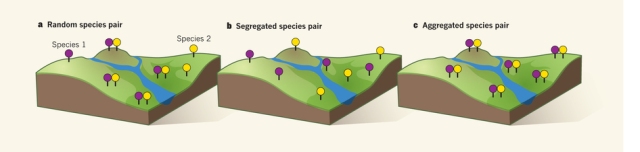
Figure 1. In the left panel, the taxa are distributed across the landscape at random; in the centre panel, the taxa don’t co-occur, they are segregated; in the right panel, the taxa are aggregated (Dietl 2016). If species were all as easy to identify as this, I could be a field ecologist. (Source Dietl 2016)

Lyons et al find that the proportion of aggregated taxon-pairs begins to change in the mid-Holocene, about 6000 years ago. This change

coincided with increasing human population size and the spread of agriculture in North America

They conclude

The organization of modern and late Holocene plant and animal assemblages differs fundamentally from that of assemblages over the past 300 million years that predate the large-scale impacts of humans. Our results suggest that the rules governing the assembly of communities have recently been changed by human activity.

The authors favoured hypothesis is that habitat fragmentation and dispersal limitation are responsible.

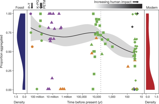
Figure 2. Changes in the proportion of aggregated taxon-pairs over the last three hundred million years. (Source Lyons et al.)

North American mid-Holocene agriculture

If mid-Holocene agriculture was responsible for changing the structure of animal and plant assemblages, one might expect that agriculture to have been intense and extensive. Zelder & Smith (2009), one of two papers by Smith cited by Lyons et al as evidence of mid-Holocene agriculture, write

Five different cultivated varieties of crop plants were brought under domestication in eastern North America between 5000 and 3800 cal. BP: squash Cucurbita pepo, sunflower Helianthus annuus var. macrocarpus, marsh elder Iva annua var. macrocarpa, and two cultivated varieties of chenopod Chenopodium berlandieri (Smith 2006). Clear evidence of the development of a crop complex based on these indigenous eastern seed plants is present by 3800 cal. BP (Smith and Yarnell 2009), but indications of a dominant subsistence role for any crop plant do not appear until after AD 700, when a widespread shift to maize‐centered agriculture is documented by a dramatic change in stable carbon isotope values in human burial populations (Smith 1990).

It would appear that the claim that agriculture at 6000 BP had fundamentally affected the ecological patterns has fallen at the first hurdle: there is no evidence of agriculture this early in eastern North America. That is not to say that humans had no impact of the landscape: just ask any giant sloth.

Poor data-set selection

Any analysis critically depends on the quality and relevance of the data to the hypothesis being tested. Unfortunately, there are serious issues with the modern data used by Lyons et al. They use:

• 53 fossil mainland data-sets
• 48 modern mainland data-sets
• 53 modern island data-sets

The modern island data are only used in the breakpoint analysis (see below) but their relevance is doubtful as different biogeographic processes are important on islands and none of the fossil data-sets are from islands. If Lyons et al were convinced that they were comparable, they would have used them throughout.

Most of the modern mainland data-sets (and all the island data) are a subset of data from a compilation by Atmar & Patterson (1995) for testing their nestedness temperature method. Gotelli & Ulrich (2010) are cited – but they just used the earlier compilation. Once I had been sent the list of data-sets used, I was able track down the metadata for each data-set. There were a large number of issues in the modern mainland data. For example,

• Two of the data-sets from the Canary Islands were mis-categorised as being mainland.
• Two data-sets were perfect duplicates of each other.
• One data-set was a transposed (taxa became sites, and vice versa) near-duplicate of another data-set (Atmar & Patterson had not stored the species or site names so this was only obvious when checking the source publication).
• Some of the data-sets were very small. The smallest island data-set had only four samples; the smallest mainland data-set had seven.

There were many overlapping data-sets. For example:

• Two data-sets of Western Australian snails differed only in how sub-species were treated.
• The bird assemblages in 12 Illinois woods sampled in 1979 and 1980 were treated as independent data-sets.
• A total of 12 data-sets covered rodents from three habitats in four deserts from the SW USA. The 45 samples from Sonoran desert scrub data-set were included in the 48 sample Sonoran all habitats data-set. They were also included in the all-desert scrub data-set and the all-desert all-habitat data-set.

These overlaps should not have been a surprise as they are documented by Wright et al (1997).

These duplicate and near duplicate data-sets will probably bias the analysis as they give more weight to these data-sets and underestimate the p-value. A similar problem occurs in the fossil pollen data which includes 1000 year time slices of the North American pollen database.

Some of the modern data-sets are from dispersal-limited systems, such as ‘sky-islands’ of boreal forest on mountains in the desert and terrestrial cave invertebrates. The logic that excludes the real island data-sets should also exclude these.

Although Lyons et al are hypothesising that human activities, especially agriculture, are responsible for the change in assembly rules, some of the included data-sets are of minimal relevance to this hypothesis, for example the cave invertebrates mentioned above and the invertebrate assemblages colonising jars of artificial lake water at different distances from a Texan lake.

Lyons et al reply

Lyons et al published a corrigendum that dealt with the mis-categorised, the completely duplicated and the transposed data-sets. It also added some accidentally omitted island/marine data-sets (marine fouling organisms on tile plates suspended underneath Duke University Marine Laboratory dock) which should have been deliberately excluded as irrelevant.

Perhaps not surprisingly, the authors disagree with our assertion that many of the modern data-sets are inappropriate for comparison with fossil data-sets.

Their main argument in this section seems to be that since the modern landscape is highly fragmented, data-sets from relict or patchy habitats should not be excluded. We did not argue that data-sets from landscapes that have been fragmented by human activity should be excluded, but that naturally dispersal limited systems, akin to islands, should be excluded for the same reason that islands are excluded. Most of the data-sets we think should be excluded as ‘islands’ are also small, so should have been excluded because they were small anyway (see below).

The authors’ rejoinder that some fossil data-sets were from edaphically distinct habitat islands is less persuasive when you look at the papers cited and see that they refer to floodplain deposits – which tend to be linear systems rather than islands.

Lyons et al re-run their analysis without small, overlapping, or dispersal limited modern data-sets and report that the results are consistent with the original results. The mean proportion of aggregated taxon pairs for the modern data-sets rose from 0.33 to 0.53 with the strictest criteria (no overlaps, n = 50) which left eight modern data-sets out of the original 50 (there was some confusion as to which data-sets had originally been included).

However, Lyons et al explicitly did not delete any pollen assemblages

because they are separated by 1,000 to 20,000 years, do not necessarily contain the same cores, and vary in their geographic extent. They are not subsets of one another, even if some of the genera and sites may recur.

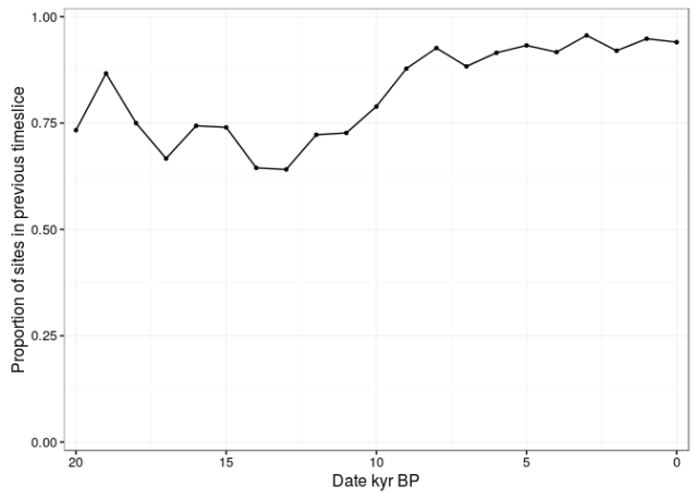
Figure 3. Proportion of pollen cores in each 1000 year time-slice that were in the previous time-slice.

For the Holocene, typically over 90% of pollen cores in each time-slice are shared with the previous time-slice. The geographic area is typically very similar between adjacent time slices. Treating each time-slice as if it is independent over-inflates the importance of the pollen data, which constitutes the vast majority of data-sets in the 100 – 100,000 year range.

The breakpoint is broken

Lyons et al use a breakpoint analysis to determine when the change in proportion of aggregated taxon pair starts. This analysis fits separate regression lines to the data either side of a breakpoint, the position of which is estimated. The breakpoint analysis gives the authors the headline result that there is a mid-Holocene change in assembly rules and hence that human activity might be responsible.

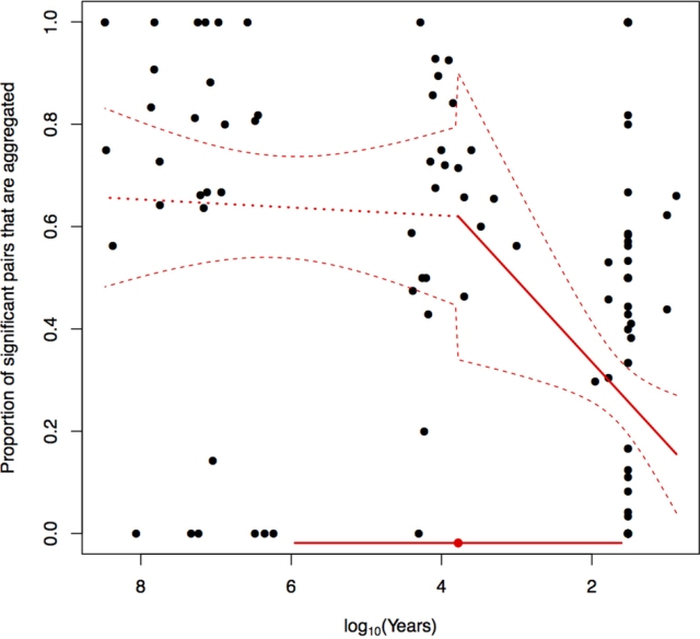
Figure 4. Breakpoint analysis from Lyons et al.

The confidence intervals in figure 4 are clearly wrong. The confidence intervals appear to be drawn for each regression line separately rather than for the model as a whole.

All the data, island and mainland, are used in the breakpoint analysis

  The breakpoint analysis was run using all the data resolved to the best possible dates to allow for the greatest amount of power in detecting where the switch occurred.

But the reader is assured that

the results were similar when island data were excluded.

The paper only reports the results with the island data included. So I asked for the results without the island data (which I think should have been given, at least in supplementary material).

With the island data included, the breakpoint occurred 5998 years ago with a 95% confidence interval of 40 – 893,000 years. This breakpoint could have occurred between the mid-Pleistocene transition and 1970. Difficult to pin this on early agriculture.

Without the island data, the breakpoint is at 5998 years and the 95% confidence interval is 7 – 4,940,000 years. So the estimate is exactly the same, even though a third of the data have been removed and the confidence interval has now extends into the mid-Pliocene.

The authors interpret the extreme stability of the estimate as evidence that the result is robust. We viewed it as an indicator of pathological behaviour in the segmented R package used. So we (or rather Joe) re-implemented the breakpoint analysis using Markov chain Monte Carlo.

Re-running the breakpoint analysis

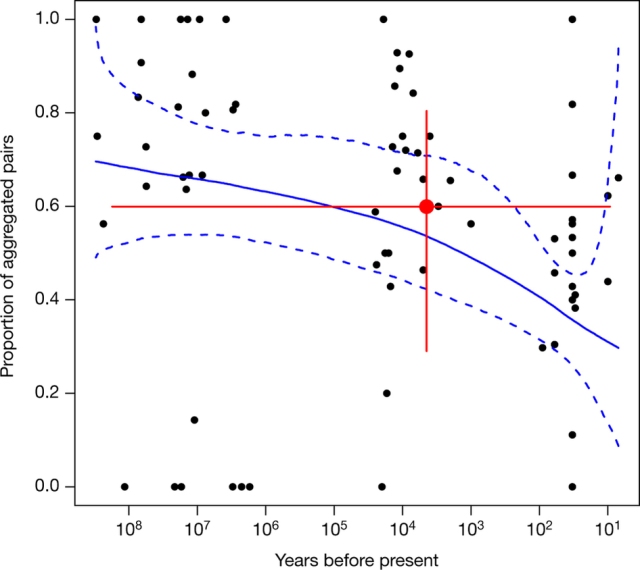
Figure 5. The result of our breakpoint analysis.

Importantly, this is the same underlying model that Lyons et al use. All that has changed is the fitting mechanism. When fitted with one breakpoint, the model finds a mid-Holocene breakpoint with extremely wide credibility intervals. However, a model with no breakpoint has lower deviance information criterion score. The timing, and indeed existence, of a breakpoint is highly uncertain. The claim of a mid-Holocene breakpoint by Lyons et al is very weak.

Lyons et al reply

Apparently we “misconstrue” the authors’ use of the break-point analysis.

We did not use it as a formal statistical hypothesis test. … Rather, we used the break-point analysis to identify the approximate time the decline became more pronounced.

Why don’t they just admit that the breakpoint analysis was flawed.

They report the most parsimonious model is one that does not have a break point but instead an “exponential decline” in the proportion of aggregated pairs through time.

This is becoming misleading. This might suggest that we are using an exponential model as an alternative to a linear model with a a breakpoint. We are not. Following Lyons et al, we use log(age) as the predictor. Since we do not find evidence for a breakpoint, we prefer the simpler no-breakpoint model. The choice by Lyons et al of an log(age) predictor has the natural consequence that any change is exponential against age. The exponential decline is not a finding of the model: it is an assumption of the model. It is not a very sensible model. For example, it is now almost a year after the paper was published: what is the predicted percent of aggregated taxon pairs? You cannot tell: log(-1) is not a number. Following their model, at age = 0, the percent aggregated taxon pairs reached minus infinity. Clearly, the domain in which the model is valid is restricted.

Contrary to what Lyons et al argue in their reply, we did not confirm that the decline is non-linear, nor that the decline becomes steeper in the Holocene. These are direct consequences of the model they selected.

It is interesting to contrast the little emphasis the authors would now give to the breakpoint with quotes from the authors in press coverage at the time the paper was published (I’m just taking quotes as other aspects of the press release might have been written by journalists).

When early humans started farming and became dominant in the terrestrial landscape, we see this dramatic restructuring of plant and animal communities. Gotelli

The fraction of plant and animal species that were positively associated with each other was mostly unchanged for 300 million years. Then that fraction sharply declined over the last 6,000 years. Waller

the study even provides a way to date the start of the anthropocene. Waller

This tells us that humans have been having a massive effect on the environment for a very long time. Lyons

The pattern of co-occurring species remained stable through the evolution of land organisms from the earliest tetrapods through dinosaurs, flowering plants and mammals. This pattern didn’t change because of previous mass extinctions or ancient climate variability, but instead, early human activities 6,000 years ago suddenly began resetting a basic property of natural communities. Behrensmeyer

But more and more, research into the Holocene and the Pleistocene is showing that when humans started migrating around the globe, they started having major, unprecedented impacts. Lyons

Biases in the statistics

Often the interesting figures that show problems with a paper are buried deep in the supplementary material. So it is with Lyons et al. The supplementary material include the presence-absence matrices for each fossil data-set and the taxon co-occurrence plot.

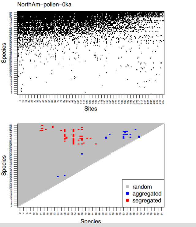
Figure 6. Upper panel – presence-absence matrix for the North America pollen 0 ka with taxa ordered by occupancy and sites ordered by richness. Lower panel – co-occurrence plot with taxa ordered by occupancy.

Many of the co-occurrence plots resemble figure 6 with aggregated and segregated taxon-pairs occupying distinct places in the plot. The general pattern is this: two very rare (bottom left) or two very common taxa (top right) cannot be identified as either aggregated or segregated as there is not enough statistical power. Segregated pairs tend to have one common and one rare taxa (top left). Aggregated pairs tend to have taxa with similar occupancies (near diagonal).

Since it is reasonable to expect aggregated and segregated taxon pairs to exist over (almost) the full range of occupancies, the observed pattern probably reflects differences in the statistical power available to detect aggregation and segregation at different levels of occupancy.

Realising there were problems with statistical power, I decided to check if the proportion of aggregated taxon pairs was affected by data-set size. I am surprised that this does not appear to have been done before. Small data-sets will have less statistical power, but will detection of aggregated and segregated pairs be equally affected? The first simple test of this is to plot the proportion of aggregated taxon pairs against data-set size.

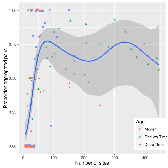
Figure 7. Proportion aggregated taxon pairs against data-set size.

There is a strong relationship between data-set size and the proportion of aggregated pairs. Very small data-sets have a low proportion of aggregated pairs. The proportion stabilises once there are more than ~50 sites in the data-set.

The relationship can be explored more directly by taking different sized random sub-samples of a large data-set (ensuring that the number of species is constant). I did this for four data-sets. There are strong, but perhaps inconsistent, patterns in each data-set.

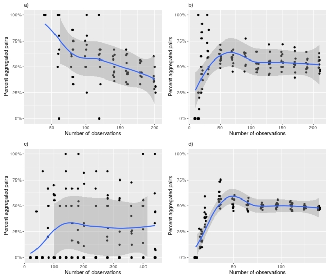
Figure 8. Effect of number of observations on percentage of aggregated taxon pairs for four data-sets used by Lyons et al. US desert rodents (a), Holocene mammals (b), 1,000-year-old North American pollen (c), and 1950 Wisconsin understorey vegetation (d). Grey band shows 95% confidence interval of a local regression smoother fitted with a quasi-binomial distribution.

Holocene mammals and Wisconsin understorey vegetation have the most similar patterns. Initially, there is little change in the proportion of aggregated taxon pairs as the data-set is reduced in size. Then there is a slight rise followed by a strong fall.

The North American pollen 1ka data-set had a similar pattern but is noisier because there are fewer non-random pairs in this data-set.

The desert rodent data-set shows only a rise in proportion aggregated pairs. Very few subsets with fewer than fifty sites had any non-random taxon pairs, so it is not possible to tell what happens for small data-sets.

Part of this inconsistency probably relates to patterns of occupancy within the data-sets.

Lyons et al reply

Lyons et al ignore figure 7 completely and focus on the inconsistent patterns shown in figure 7. Yes the patterns are inconsistent – but probably understandable with more work – but the existence of any pattern with data-set size should worry the authors.

They claim that the effect is only found with very small samples

Using data from Telford et al. simulations, we note that the purported sample size effect in their extended data fig. 1 is found only at low sample sizes (rarefying to ten samples). Even slightly elevated sampling removes this effect; when rarefying to 20, two datasets were non-significant and two showed a relationship in the opposite direction.

They are tying to fit a linear trend to data with a non-linear relationship. Not a cunning plan.

Lyons et al repeat their analyses without the small data-sets and report that the

Redoing our analyses while eliminating datasets with less than 10, 20 or even 50 sites does not change our results substantially (Extended Data Table 1).

With the n = 50 criterion, which will remove most of the sample size bias, only eight modern mainland data-sets remain out of the initial fifty. When I subset the data – it is in the supplementary material – I find nine data-sets meet the criteria.

library(readxl)
library(dplyr)
lyons <- read_excel("nature20097-s1.xlsx")

modern <- lyons %>%
filter(numSites >=50, age <= 100, land.island.ete.corrected != "island", land.island.ete.corrected.overlapping.removed != "NA") %>%
select(Dataset, numSites, percAgg)

knitr::kable(modern)

Dataset                              numSites     percAgg

———————–  ———  ———-
crypticTaxa                                    171   0.66
NorthAm-mammals-Modern    67   0.41
WI-overstory-SPP-1950           168   0.53
WI-understory-SPP-1950          152   0.46
WI-overstory-SPP-2000           168   0.62
WI-understory-SPP-2000         152   0.44
NorthAm-pollen-0ka                 252   0.30
swusrodco.txt                               202   0.53
wausnailco.txt                                 55   0.82

However, this includes two pairs of data-sets that were resampled and should have been excluded under the no overlaps criterion. That leaves just seven modern data-sets. The analysis will be very sensitive to the properties of these data-sets.

Next Lyons et al stratify the data-sets into three groups:

Deep Time (>1 million years ago; n = 29 data sets), Shallow Time (1 million–100 years ago; n = 24), and Modern (<100 years ago; n = 46).

They argue that the deep time and modern have similar data-set sizes, but differ in the proportion of aggregated taxa and hence our objections are ill founded. I’m not going to criticise what they do here, except to note that they appear to have done a t-test which won’t perform well with the non-normally distributed number of sites and that a Wilcoxon test is significant at the p = 0.05 level. I will quote this though:

Third, in re-testing for a Holocene shift, Bertelsmeier and Ollier … break the data into three arbitrary time bins that bear no correspondence to accepted geological time periods. Their ‘ancient’ is 300 million years ago to 1 million years ago, which encompasses two of the largest recorded mass extinctions, the break-up of Pangaea, considerable changes in climate, the rise of angiosperms and a change from dinosaur- to mammal-dominated terrestrial ecosystems. Moreover, their definitions merge all Pleistocene and non-modern Holocene data into a single bin, obscuring a Holocene shift.

What drives aggregated and segregated taxon pairs

Non-random co-occurrence patterns can be driven by a variety of factors.

• Large scale dispersal limitations (polar bears and walrus vs penguins)
• Niche separation (polar bears vs pandas)
• Biotic interactions (mutalists, competitive exclusion)
• Small scale dispersal limitations (between islands, habitat fragments)

Because of the large spatial scale of some the data-sets in Lyons et al, niche separation is important, but probably little affected by human activity. For example, looking closely at the North American pollen 0ka slice (figure 5) we see that of the 48 segregated pairs, 13 (27%) include Rhizophora (species 33, red mangrove). Rhizophora is only found in Florida mangrove swamps and does not co-occur with temperate and boreal trees. Humans have not altered this relationship, but because Rhizophora only occurs in the most recent two pollen time-slices (probably due to sea-level rise submerging early Holocene mangrove swamps), it contributes to the apparent decrease in the proportion of aggregated taxon pairs.

Conclusions

It is exciting to see palaeoecological data being used to address important ecological questions, but devastating that such bold claims are supported by inappropriate data and analyses.

Given the number and severity of problems with Lyons et al (2016), we thought that they might retract the paper. Instead they essentially admit to all the problems, but carry on regardless.